Survival Analysis and Hazard Models

Wooyong Park

Hazard Model

Introduction to hazard models

Hazard models are better than the traditional regression approach.

The traditional regression approach specifies a probability distribution for the duration time and fits it using data. The hazard approach, on the other hand, determines the probability of the outcome as a sequence of simpler conditional events.

(Conditional sequential probabilities vs Unconditional direct probability distribution)

Model Intuition

Let \(\lambda = \lambda(X_i, t)\) denote the probability of a certain spell being terminated.
Such probability of adoption/termination would typically be affected by individual characteristics(\(X_i\)) and the duration of the spell(\(t\)).
e.g. Probability of the spell being terminated in exactly 5 weeks: \(\left(1-\lambda(X_i,t)\right)^4 \cdot \lambda(X_i,t)\)

Hazard Functions

Hazard Function

\[\lambda(u) = \frac{P(u < t \leq u+\delta u|t>u)}{\delta u}\] Meaning) Given that the spell wasn’t lifted by \(t = u\), the probability of the spell being lifted in \(\delta u\) divided by the interval, \(\delta u\).

Hazard Functions

Classical Distribution(Unconditional Distribution)

Note that \(P(u\leq t)\) is the CDF of the time from the beginning of the spell to the termination of the spell. Denote it by \(F(t)\). Then,

\[\begin{align} \lambda(u) &= \frac{P(u < t \leq u+\delta u|t>u)}{\delta u}\\ &=\frac{P(t \leq u+\delta u) - P(t \leq u)}{\delta u \times P(t>u)}\\ &=\frac{1}{1-F(u)}\cdot\frac{F(u+\delta u)-F(u)}{\delta u} \stackrel{\delta u \to 0^{+}}{=}\frac{f(u)}{1-F(u)} \end{align}\]

Relationship between hazard functions and classical distribution

Kiefer(1988) states that every hazard function has an exact mathematical equivalent in terms of an unconditional probability distribution.
By solving the differential equation,

\[f(u) = \lambda(u)\cdot exp\left[-\int_0^u \lambda(s)ds \right]\]

Survivor Function

The survivor function is defined as \(S(u) = 1-F(u)\).
(i.e. the probability of spell being sustained until \(t=u\))
Thus,

\[\begin{align} \lambda(u) &= \frac{f(u)}{1-F(u)}\\ &= \frac{f(u)}{S(u)} = \frac{dF/du}{S(u)}\\ &= \frac{-dS/du}{S(u)} = -\frac{dlnS(u)}{du} \end{align}\] Here, we can think of the survivor function as the endurance probability of a spell.

RMK) Notice that if we could consistently estimate \(S(u)\), we can also consistently estimate \(\lambda(u)\) given that differentiability and continuity of the derivative are guaranteed.

Parametric Hazard

Parametric vs Nonparametric

Parametric Hazard: Specifies the functional form of hazard before estimation
Nonparametric/Semiparametric Hazard: does not specify the hazard function form

1. Constant Hazard

definition: \(\lambda(u) = \lambda_0\) for all \(u>0\).
unconditional pdf: \(f(u) = \lambda_0 exp\left[-\lambda_0 u\right]\)
\(\to\) exponential distribution with rate parameter \(\lambda_0\)

RMK) Notice that rate parameters describe the frequency or intensity of a random event in a unit time, which is equivalent to how we defined the hazard function itself.

Parametric Hazard

2. Weibull Distribution

Weibull distribution permits a monotonically increasing/decreasing hazard function, which either describes the “snowballing” effect or the “inerital” effect. Weibull survival functions are determined by two parameters: \(\alpha\) and \(\sigma\).

definition: \(\lambda(u) = \lambda(u) = \sigma \alpha (\sigma u)^{\alpha-1}\) s.t. \(\sigma>0\) and \(\alpha>0\)
unconditional pdf: \(f(u) = \sigma \alpha (\sigma u)^{\alpha-1}(1-\sigma u)\)
Monotone Increasing(\(\alpha>1\)), Monotone Decreasing(\(\alpha<1\)), Constant Hazard(\(\alpha = 1\))

3. Log-Normal Distribution

The log-normal model assumes that the log of a survival time follows a normal distribution. Such model allows the hazard to be non-monotonic.

Nonparametric Hazard

The problem with parametric methods is that under misspecified models(i.e. misspecified functional form of the hazard), the estimator is inconsistent of the actual hazard. Also it is often the case that the underlying model is difficult to specify. In such cases, we can rely on nonparametric hazard estimations.

Cox PH Model

Among multiple nonparametric approaches, we only cover the Cox proportional-hazards model. Cox (1972) proposes a model that doesn’t require the distribution of survival durations to be known, at the cost of not estimating the hazard function itself.

However, it is actually a semi-parametric approach in that it assumes a functional form in the regression on exogenous variables, which will be discussed shortly.

Incorporation of Exogenous Variables

Cox PH Model

From now on, we denote the hazard function \(\lambda(u)\) by \(h(t)\) instead.

\[ h_i(t) = h_0(t)exp\left[\beta_1X_{i1} +\cdots +\beta_kX_{ik}\right]\]

\(h_0(t)\)
: the baseline hazard \(\to\) doesn’t require functional form
\(exp(\sum_{j=1}^k\beta_jX_{ij})\)
: effects of covariates \(\to\) specifying the functional form

Regression Coefficient

\[\log h_i(t) = \log h_0(t) + \beta_1X_{i1} + \cdots + \beta_kX_{ik}\]

\(\beta_j = \frac{\partial \log h_i(t)}{\partial X_{ij}}\), which means that the regression coefficient is the partial derivative of the log-hazard w.r.t. the covariate.

(Equivalently, \(\beta_j\) denotes the percentage change of the hazard w.r.t. the unit change of the covariate)

Cox PH Model

\[ h_i(t) = h_0(t)exp\left[\beta_1X_{i1} +\cdots +\beta_kX_{ik}\right]\]

\(h_0(t)\)
: the baseline hazard \(\to\) doesn’t require functional form
\(exp(\sum_{j=1}^k\beta_jX_{ij})\)
: effects of covariates \(\to\) specifying the functional form

Hazard Ratios

We show two different definitions of hazard ratios depending on the context, although they are closely related to each other.

\(exp(\beta_j)\) : the exponential transformation of the coefficient
\(\frac{\text{hazard in group A}}{\text{hazard in group B}} = e^{(X_{iA}-X_{iB})'\beta_i}\) : hazard ratio between two groups

RMK) The PH model assumes that this ratio is constant, and one group’s (or individual’s) hazard is proportional and time-independent to the other.

Proportionality Assumption(PH Model)

The Cox PH model assumes that the hazard ratio is constant. Suppose there are two individuals \(p\) and \(q\). Then,

\[\begin{align} \begin{cases} h_p(t) = h_0(t)e^{X_{p}'\beta}\\ h_q(t) = h_0(t)e^{X_{q}'\beta} \end{cases} \end{align}\]

which implies

\[\begin{align} \text{hazard ratio} = exp\left[(X_p-X_q)'\beta\right] \end{align}\]

that the hazard ratio is independent of the baseline hazard and time. Equivalently, the log-hazard ratio(\(\log h_p(t) - \log h_q(t)\)) is also constant.

Cox PH Model

\[ h_i(t) = h_0(t)exp\left[\beta_1X_{i1} +\cdots +\beta_kX_{ik}\right]\]

\(h_0(t)\)
: the baseline hazard \(\to\) doesn’t require functional form
\(exp(\sum_{j=1}^k\beta_jX_{ij})\)
: effects of covariates \(\to\) specifying the functional form

Limitations

Proportionality might not always be satisfied. In this case we adhere to the nonproportional Cox model.
cannot predict the survival time itself, nor can it provide the hazard function.

Estimation

We estimate the coefficients through partial likelihood estimation(ple). PLE is equivalent to MLE, but we only consider the likelihoods of the data that experienced the event.

In the data of observations with their spell ended, we are seeing that particular observation’s spell ended at a given time while other else’s spells could have ended at that time also. The likelihood could be described by the next question:

“Given that the spell lift happened at time \(u\), what’s the probability that it happened to the individual \(A\)?”

\[\begin{align} L_A &= \frac{h_A(u)}{\sum_{i\text{'s spell not ended before u}}h_i(u)}\\ &=\frac{h_0(t)e^{\beta_1X_{A1}+\cdots+\beta_kX_{Ak}}}{h_0(t)(e^{\beta_1X_{A1}+\cdots+\beta_kX_{Ak}} +\sum_{i(\neq A)\text{'s spell not ended before u}}e^{\beta_1X_{i1} +\cdots + \beta_kX_{ik}})}\\ &=\frac{e^{\beta_1X_{A1}+\cdots+\beta_kX_{Ak}}}{e^{\beta_1X_{A1}+\cdots+\beta_kX_{Ak}} +\sum_{i(\neq A)\text{'s spell not ended before u}}e^{\beta_1X_{i1} +\cdots + \beta_kX_{ik}}} \end{align}\]

Censoring Issues

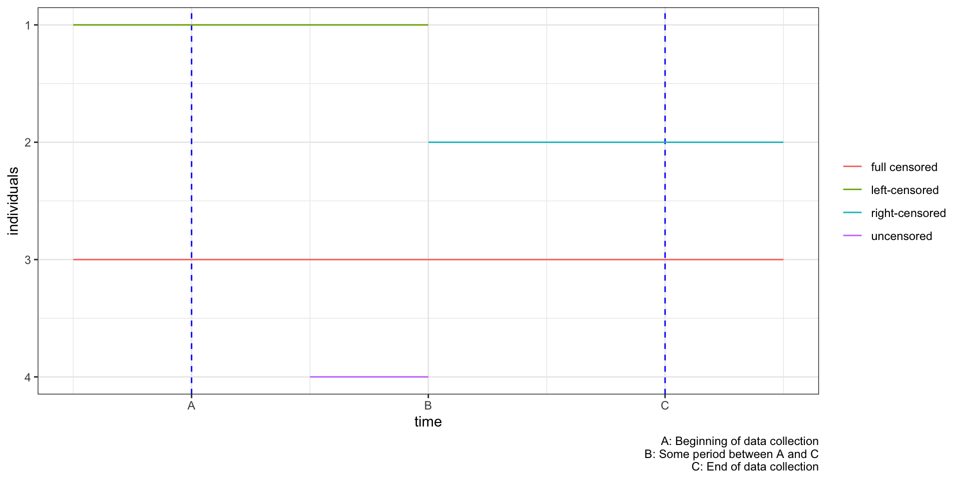
Censoring issues are what could happen in the data we hold. It indicates the event(lift of the spell) not being observed for some individuals within the study time period. We call such individuals censored observations. This problem arises may arise in three possible ways:

Left Censoring
Right Censoring
Full Censoring

However, note that in the case of right censoring, it doesn’t dissipate all valuable information, but sheds light on the information of survival probability for a given duration.

R Survival Analysis

Setting up

library(tidyverse)
library(survival)      # for survival analysis
library(survminer)     # for visualization of the analysis

All the codes and exercise materials are from STHDA.

Cox PH Model

`coxph`

coxph(formula, data, ties) helps create the Cox proportional hazard regressions in R.

formula: Linear model with a survival object as the response variable. Survival object is created using the function Surv() as follow: Surv(time, event).
data: the data
ties: used to specify how to handle ties(the default option efron is usually the most preferred)

`Surv`

Surv(time, event)

time: Follow up time
event: normally 0=alive, 1=dead

Cox PH Model

Exercise(Lung Cancer)

data('lung')
head(lung)

  inst time status age sex ph.ecog ph.karno pat.karno meal.cal wt.loss
1    3  306      2  74   1       1       90       100     1175      NA
2    3  455      2  68   1       0       90        90     1225      15
3    3 1010      1  56   1       0       90        90       NA      15
4    5  210      2  57   1       1       90        60     1150      11
5    1  883      2  60   1       0      100        90       NA       0
6   12 1022      1  74   1       1       50        80      513       0

time: Survival time in days
status: censoring status 1=censored, 2=dead
sex: Male=1 Female=2

Univariate Cox Regression

res.cox <- coxph(Surv(time, status) ~ sex, data = lung)
summary(res.cox)

Call:
coxph(formula = Surv(time, status) ~ sex, data = lung)

  n= 228, number of events= 165 

       coef exp(coef) se(coef)      z Pr(>|z|)   
sex -0.5310    0.5880   0.1672 -3.176  0.00149 **
---
Signif. codes:  0 '***' 0.001 '**' 0.01 '*' 0.05 '.' 0.1 ' ' 1

    exp(coef) exp(-coef) lower .95 upper .95
sex     0.588      1.701    0.4237     0.816

Concordance= 0.579  (se = 0.021 )
Likelihood ratio test= 10.63  on 1 df,   p=0.001
Wald test            = 10.09  on 1 df,   p=0.001
Score (logrank) test = 10.33  on 1 df,   p=0.001

Statistical Significance: determined by Wald-type tests on the likelihood induced regression coefficients
Regression Coefficients: percentage change of the hazard w.r.t. the unit change in the explanatory variable.
exp(coef): hazard ratios

Multivariate Cox Regression

res.cox <- coxph(Surv(time, status) ~ age + sex + ph.ecog, data =  lung)
summary(res.cox)

Call:
coxph(formula = Surv(time, status) ~ age + sex + ph.ecog, data = lung)

  n= 227, number of events= 164 
   (1 observation deleted due to missingness)

             coef exp(coef)  se(coef)      z Pr(>|z|)    
age      0.011067  1.011128  0.009267  1.194 0.232416    
sex     -0.552612  0.575445  0.167739 -3.294 0.000986 ***
ph.ecog  0.463728  1.589991  0.113577  4.083 4.45e-05 ***
---
Signif. codes:  0 '***' 0.001 '**' 0.01 '*' 0.05 '.' 0.1 ' ' 1

        exp(coef) exp(-coef) lower .95 upper .95
age        1.0111     0.9890    0.9929    1.0297
sex        0.5754     1.7378    0.4142    0.7994
ph.ecog    1.5900     0.6289    1.2727    1.9864

Concordance= 0.637  (se = 0.025 )
Likelihood ratio test= 30.5  on 3 df,   p=1e-06
Wald test            = 29.93  on 3 df,   p=1e-06
Score (logrank) test = 30.5  on 3 df,   p=1e-06

Vizualizing Survival Probabilities

Recall that \(h(u) = -\frac{dlnS(u)}{du}\), which implies

\[\begin{align} S(t) &= e^{-\int_0^th(u)du}\\ &=e^{-\int_0^th_0(u)exp(X'\beta)du}\\ &=e^{-\int_0^th_0(u)du \cdot exp(X'\beta)}\\ &= S_0(t)^{exp(X'\beta)} \end{align}\]

To estimate such survival probabilities and plot them, we first need the baseline hazard and the following baseline survivability via other methods.

Visualizing Survival Probabilities

In the survival package, the baseline survival and hazard are first estimated by the Breslow estimator.

Base Hazard

base_hazard <- basehaz(res.cox)
head(base_hazard)

       hazard time
1 0.003963022    5
2 0.015948084   11
3 0.019992796   12
4 0.028188936   13
5 0.032333588   15
6 0.036493082   26

Base Survivability

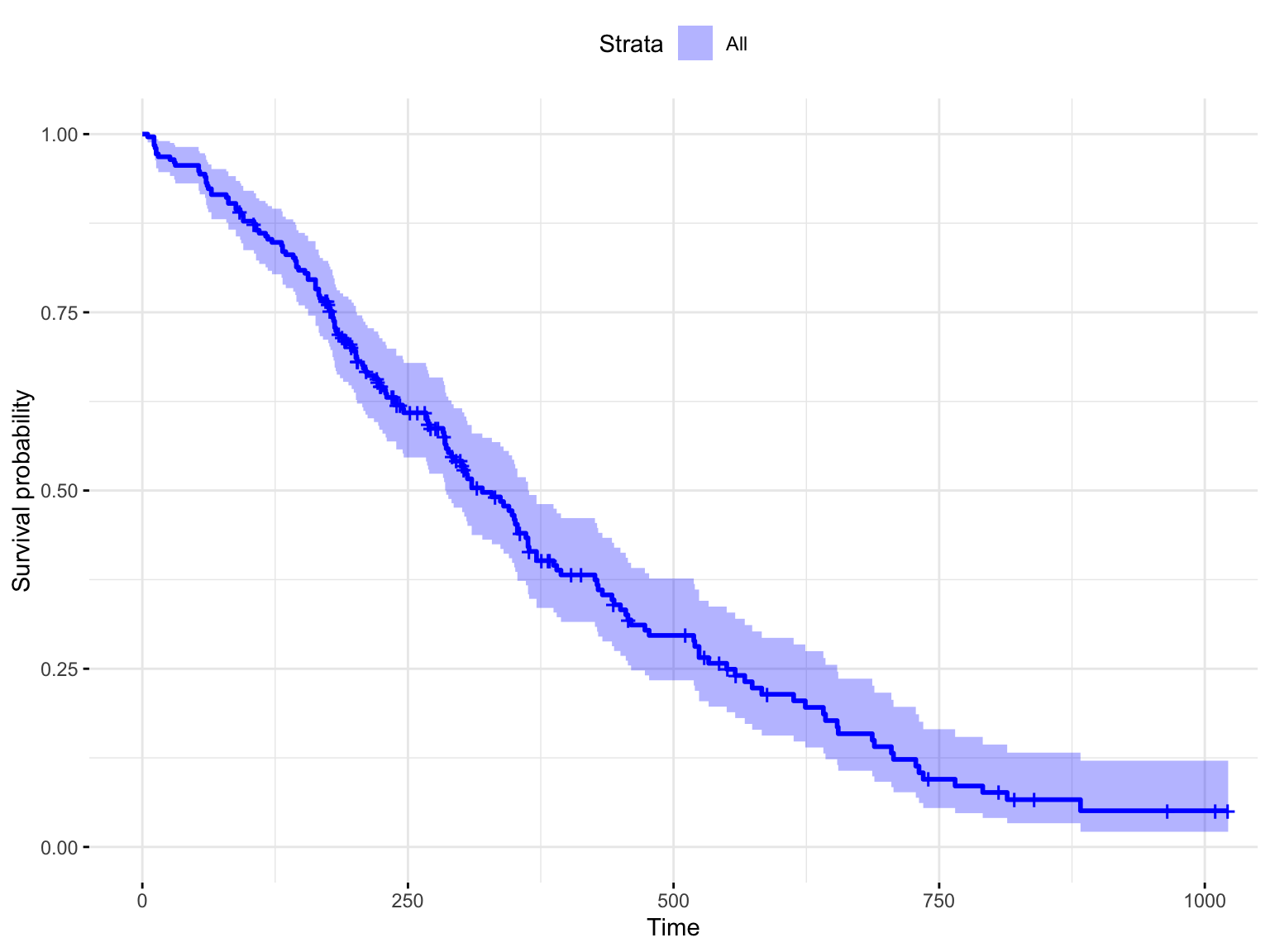
ggsurvplot(survfit(res.cox), data = lung, color = 'blue', ggtheme = theme_minimal())

Visualizing Survival Probabilities

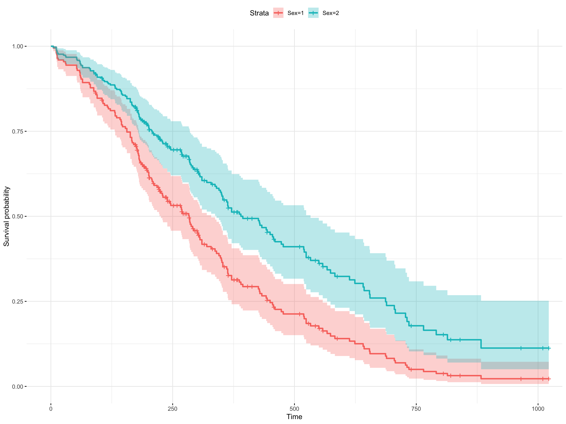
Group level Survivability

# Create the new data  
sex_df <- with(lung,
               data.frame(sex = c(1, 2), 
                          age = rep(mean(age, na.rm = TRUE), 2),
                          ph.ecog = c(1, 1)
                          )
               )
# Survival curves
fit <- survfit(res.cox, data = lung, newdata = sex_df)

ggsurvplot(fit, conf.int = TRUE, legend.labs=c("Sex=1", "Sex=2"),
           ggtheme = theme_minimal())