Recursive Partitioning
for Heterogeneous Causal Effects

Susan Athey and Guido Imbens(2016)

Wooyong Park, Joonwoo Shin, Jeongwoo Yang, Minseo Seok

URL - wooyongp.github.io/rpart-jsc25_1/slides.html

Data-driven HCE analysis based on tree models

Don’t stress. We are going to start from scratch.

Causal Inference with binary treatment

Research Question:

Does a smile in your online profile help your online micro-borrowing?(Athey et al, 2022 NBER WP)

  • W_i \in \{0,1\} : Your treatment status

Under SUTVA(Stable Unit Treatment Values Assumption),

  • Y_i(1) : individual i’s potential outcome if he/she smiled
  • Y_i(0) : individual i’s potential outcome if he/she did not

Your treatment effect is the difference between the two: \tau_i = Y_i(1) - Y_i(0)

Missing Counterfactuals and ATE

What we see:

Y_i = W_iY_i(1) + (1-W_i)Y_i(0)

Since we cannot observe both situations, we usually rely on ATE:

\tau = \mathbb{E}\bigl[Y_i(1)-Y_i(0)\bigr]

If

        1. the treatment is randomized

        2. the treatment is uncorrelated with unobserved characteristics

        3. we have an IV

we can unbiasedly estimate the ATE.

Heterogeneous Treatment Effects

Limitations of ATE

Sometimes, the ATE is insufficient.

Unfortunately, some people’s smiles might not be as alluring as others’. \rightarrow HTE


Conditional ATEs

CATE tries to explain them within the data:

\tau(X_i) = \mathbb{E}\bigl[Y_i(1) - Y_i(0)|X_i\bigr]

Athey and Imbens(2016): Tree-based model, a ML algorithm, can hint on how to choose X_i

Key concepts in ML

In terms of prediction, OLS(\mathrm{y}=X'\beta +\varepsilon) is not good enough.

  1. Not all DGPs are linear.

  2. Bias-Variance tradeoff in Prediction

\begin{align*} \text{Prediction Error} &=\mathbb{E}\bigl[\bigl(f(x)+\varepsilon-\hat{f}(x)\bigr)^2\bigr]\\ & = \underbrace{\mathbb{E}[f-\hat{f}]^2}_{\text{bias}} + \underbrace{\mathbb{V}(\hat{f})}_{\text{variance}} + \mathbb{V}(\varepsilon) \end{align*}

The unbiased predictor is not usually the minimum-error predictor, but most models/estimations including OLS focus on unbiasedness!

Why important? Heterogeneity in TE can be nonlinear wrt X.

Building a Tree

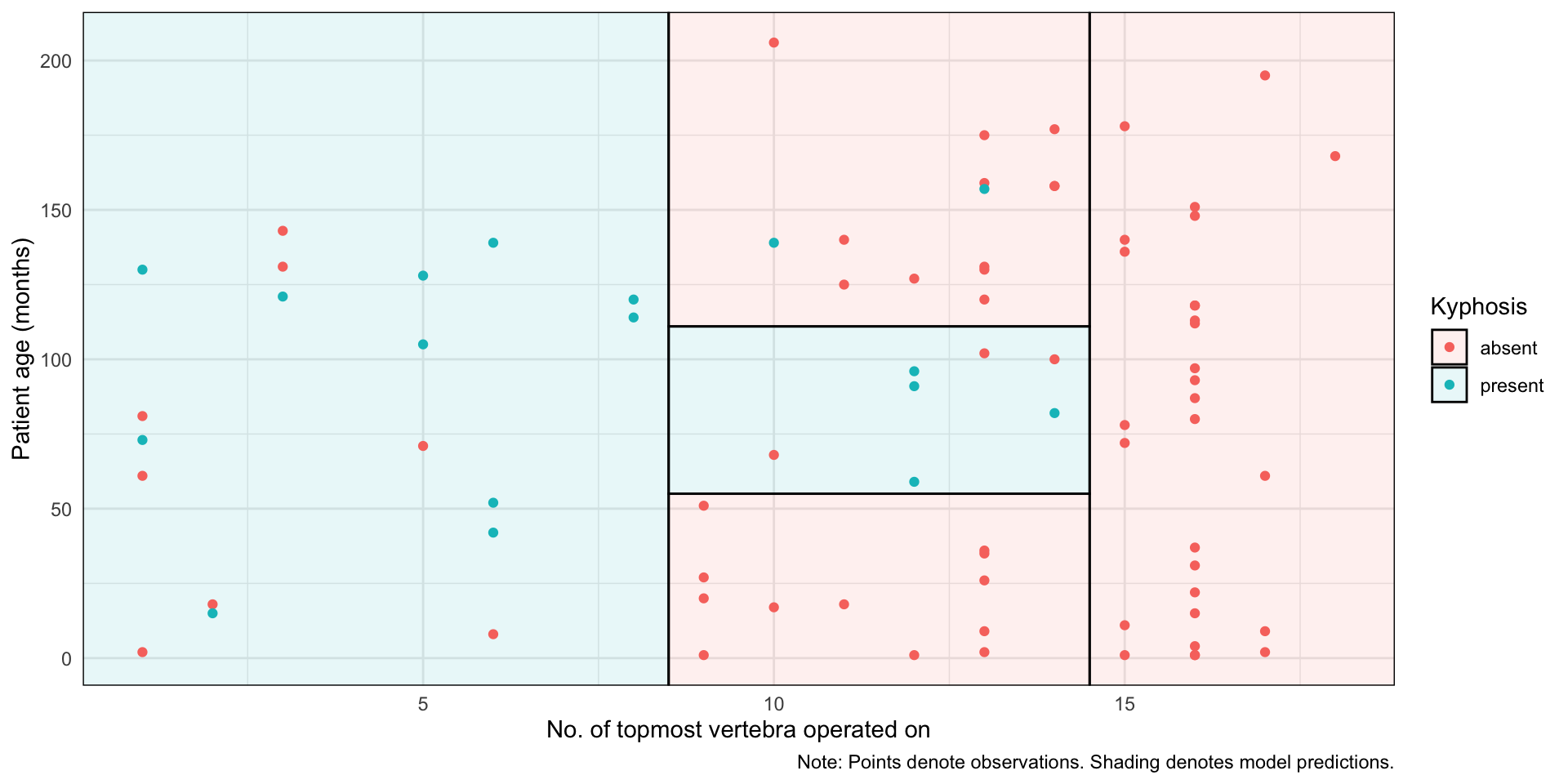
Classification and Regression Trees recursively divide the covariate space into two so that MSE decreases each time we add a partition. In the figure below, we have a partition with 5 leaves.

Code
# See the full code at Grant Mcdermott's repository
library(rpart) 
library(parsnip)
library(tidyverse)
library(parttree)
set.seed(123) ## For consistent jitter

fit = rpart(Kyphosis ~ Start + Age, data = kyphosis)

ggplot(kyphosis, aes(x = Start, y = Age)) +
  geom_parttree(data = fit, alpha = 0.1, aes(fill = Kyphosis)) + # <-- key layer
  geom_point(aes(col = Kyphosis)) +
  labs(
    x = "No. of topmost vertebra operated on", y = "Patient age (months)",
    caption = "Note: Points denote observations. Shading denotes model predictions."
    ) +
  theme_minimal()

Steps

  1. Choose X_1 or X_2.
  2. Choose the cutoff for dividing.
  3. Repeat these steps.
  • Trees recursively partition the covariate space so that MSE decreases each time we add a partition.

Figure from Beaulac and Rosenthal(2019)

For regression trees, the criterion for choosing covariate and a cutoff pair is the MSE.

  1. Split the data into S^{tr}(training) and S^{te}(test).

  2. Within S^{tr}, choose X_i and a cutoff k that minimizes MSE:

MSE = \underbrace{\sum_{i \in L}(y_i-\hat{y}_L)^2}_{\text{left-side MSE}} + \underbrace{\sum_{i \in R}(y_i-\hat{y}_R)^2}_{\text{right-side MSE}}

  1. Repeat this process.

  2. (Important!!) Our prediction within each leaf is the sample mean within each leaf:

\hat{y}(\text{leaf}) = \overline{y}_{(\text{leaf})}

  1. The resulting MSE of the model given a data S and partition \Pi would be MSE_\mu(S, S^{tr}, \Pi) = \frac{1}{\#(S)} \sum_{i \in S} \biggl[Y_i -\hat{\mu}(X_i; S^{tr}, \Pi)\biggr]^2

In this paper, we use the adjusted MSE: MSE_\mu(S, S^{tr}, \Pi) = \frac{1}{\#(S)} \sum_{i \in S} \biggl[(Y_i -\hat{\mu}(X_i; S^{tr}, \Pi))^2- {\color{blue}Y_i^2}\biggr]

which does not affect the splitting mechanism but makes the algebra more interpretable.

CART - Best predictor, but biased

Code
# Load required library
library(rpart)
library(ggplot2)
library(rpart.plot)

set.seed(456)

# simulate data and apply CART with two features
n <- 10000

x1 <- runif(n, 0, 10)
x2 <- runif(n, -5, 5)
y <- 1 + 2 * x1 + 3 * x2 * as.numeric(x2>0) + rnorm(n, 0, 1)  # True relationship: y = 1 + 2 x1 + 3 x2*I(x2>0) + noise
    
# Fit regression tree
data <- data.frame(x1 = x1, x2 = x2, y = y)
tree_model <- rpart(y ~ x1 + x2, data = data, control = rpart.control(cp = 0.04))
    
# Pruning
best <- tree_model$cptable[which.min(tree_model$cptable[,"xerror"]),"CP"]
pruned_tree <- prune(tree_model, cp=best)

rpart.plot(pruned_tree, digits=3)

Code
# Load required library
library(tidyverse)

# Make a data and compute the sample mean in each leaf
n <- 100000

x1 <- runif(n, 0, 10)
x2 <- runif(n, -5, 5)
y <- 1 + 2 * x1 + 3 * x2 * as.numeric(x2>0) + rnorm(n, 0, 1)  # True relationship: y = 1 + 2 x1 + 3 x2*I(x2>0) + noise

data <- tibble(x1 = x1, x2 = x2, y = y) |> 
    mutate(leaf = case_when(
        x1<2.62 & x2<1.77 ~ "1",
        x1<5.23 & x1>=2.62 & x2<1.77 ~ "2",
        x1<5.23 & x2>=1.77 ~ "3",
        x1>=5.23 & x2<1.81 ~ "4",
        x1>=5.23 & x2>=1.81 ~ "5"
    ))

df <- data |> group_by(leaf) |> summarize(unbiased_mean = mean(y)) |> 
    mutate(tree_mean = c(4.27, 9.51, 16.5, 16.9, 26.5))

kableExtra::kable(df)
leaf unbiased_mean tree_mean
1 4.334393 4.27
2 9.563450 9.51
3 16.405273 16.50
4 17.000677 16.90
5 26.452853 26.50

Roadmap

Trees can be more flexible and data-driven. However,

  • CART - biased estimates of CATE \rightarrow \mathbb{E}[\hat{\tau}(X;S^{tr}) \mid x] \neq \tau(x)
  • How to solve? We split the sample
    • S^{tr} for building a tree
    • S^{est} to estimate CATEs and take no role in building a tree
  • How does this change the tree?
    • For outcome prediction(Y) - Joonwoo
    • For CATE(\tau(X)) - Jeongwoo
    • Simulation Results - Minseo

Honest Inference for Outcome Averages

Notations for predicted outcomes

  • Given a partition \Pi, conditional mean is given by: \begin{equation*} \mu(x;\Pi) = \mathbb{E}\left[Y_i | X_i \in \textit{l}(x;\Pi)\right] \end{equation*}

  • Given a sample \mathcal{S} we estimate conditional mean is given by \begin{equation*} \hat{\mu}(x;\mathcal{S},\Pi) = \frac{1}{\#(i \in \mathcal{S} : X_i \in \textit{l}(x;\Pi))}\sum\limits_{i \in \mathcal{S}:X_i \in \textit{l}(x;\Pi)}Y_i \end{equation*}

Limitations of CART

We cannot simply use CART to estimate HTE.

  • Potential bias in the leaf estimates
  • does not consider variance in tree splitting

Limitations of CART

Suppose Y_i \in \mathbb{R}, \quad X_i \in \{L,R\}

  • Only two possible partitions : \begin{equation*} \Pi = \begin{cases} \{L,R\} & (\text{no split}) \\ \{ \{L\}, \{R\} \} & (\text{split}) \end{cases} \end{equation*}

  • To build Regression tree, we compare

\begin{align*} &\frac{1}{\#(S^{tr})}\sum\limits_{i: X_i \in S^{tr}}(Y_i-\bar{Y})^2 \quad\text{and}\qquad \qquad \\ &\frac{1}{\#(S^{tr})}\biggl[\sum\limits_{i: X_i=L}(Y_i-\bar{Y_L})^2+\sum\limits_{i:X_i = R}(Y_i-\bar{Y_R})^2\biggr] \end{align*}

Limitations of CART

  • This is equivalent to

\begin{align*} \pi(S)= \begin{cases} \quad \{ \{L,R \} \} & \text{if} \quad |\bar{Y}_L -\bar{Y}_R| \leq c \\ \quad \{ \{L\}, \{R \} \} & \text{if} \quad |\bar{Y}_L -\bar{Y}_R| > c \end{cases} \end{align*}

If we condition on \left|\bar{Y}_L -\bar{Y}_R\right| > c, we expect bias:

\mathbb{E}(\overline{Y}_k) \neq \mathbb{E}(\overline{Y}_k| \left|\overline{Y}_L -\overline{Y}_R \right| > c)

where k \in \{L,R\}

Limitations of CART

Example

Code
# See the full code at Grant Mcdermott's repository
library(rpart) 
library(parsnip)
library(tidyverse)
library(parttree)

train1 <- kyphosis %>% head(50)
estimation <- kyphosis %>% tail(31)
set.seed(456) ## For consistent jitter
train2 <- kyphosis %>% sample_n(50)

fit = rpart(Kyphosis ~ Start + Age, data = train1)

ggplot(train1, aes(x = Start, y = Age)) +
  geom_parttree(data = fit, alpha = 0.1, aes(fill = Kyphosis)) + # <-- key layer
  geom_point(aes(col = Kyphosis)) +
  labs(
    x = "No. of topmost vertebra operated on", y = "Patient age (months)",
    caption = "Note: Points denote observations. Shading denotes model predictions."
    ) +
  theme_minimal()

Code
fit = rpart(Kyphosis ~ Start + Age, data = kyphosis)

ggplot(kyphosis, aes(x = Start, y = Age)) +
#   geom_parttree(data = fit, alpha = 0.1, aes(fill = Kyphosis)) + # <-- key layer
  geom_jitter(aes(col = Kyphosis)) +
  geom_point(aes(x=10, y=50), color = "#F8766D") +
  geom_point(aes(x=3, y=58), color = "#F8766D") +
  geom_point(aes(x=12.3, y=210), color = "#F8766D") +
  geom_point(aes(x=12.2, y=200), color = "#F8766D") +
  geom_point(aes(x=4, y=65), color = "#F8766D") +
  geom_point(aes(x=4.5, y=100), color = "#F8766D") +
  geom_segment(aes(x = 0, xend = 12.5, y = 35, yend = 35), linetype="dashed") +
  geom_vline(aes(xintercept=12.5), linetype="dashed") +
  labs(
    x = "No. of topmost vertebra operated on", y = "Patient age (months)",
    caption = "Note: Points denote observations. Shading denotes model predictions."
    ) +
  theme_minimal()

CART vs Honest

Honest Estimation uses two different samples : S^{tr} for splitting and S^{est} for estimation.

CART

\hat{\mu}(x;S^{tr},\pi(S^{tr}))=\frac{1}{\#(i \in S^{tr} : X_i \in \textit{l}(x;\pi(S^{tr})))}\sum\limits_{i\in S^{tr}:X_i \in \textit{l}(x;\pi(S^{tr}))}Y_i

Honest

\hat{\mu}(x;{\color{red}S^{est}},\pi(S^{tr}))=\frac{1}{\#(i \in {\color{red}S^{est}} : X_i \in \textit{l}(x;\pi(S^{tr})))}\sum\limits_{i\in {\color{red}S^{est}}:X_i \in \textit{l}(x;\pi(S^{tr}))}Y_i

The Honest Criterion

\begin{align*} \text{MSE}_{\mu}(\underbrace{S^{tr}}_\text{training set},\underbrace{S^{est}}_\text{estimation set},\Pi) &= \frac{1}{\#(S^{tr})}\sum\limits_{i \in S^{tr}}\left[(Y_i - \hat{\mu}(X_i;{\color{red}S^{ est}},\Pi))^2-Y_i^2\right] \end{align*}

\begin{align*} \text{EMSE}_\mu &= \mathbb{E}_{S^{tr},S^{est}}\left[\text{MSE}_\mu(S^{tr},S^{est},\Pi)\right] \end{align*}

where the expectation is taken over all possible S^{tr} \quad and S^{est}.

The Honest Target

  • Given \Pi, we can expand EMSE_\mu(\Pi) :

\begin{align*} -\text{EMSE}_\mu(\Pi) &= -\mathbb{E}_{(Y_i,X_i),S^{est}}\left[(Y_i-\mu(X_i;\Pi))^2 - Y_i^2\right] \\ &\quad-\mathbb{E}_{X_i,S^{est}}\left[(\hat{\mu}(X_i;S^{est},\Pi)-\mu(X_i;\Pi))^2\right]\\ &\quad= \mathbb{E}_{X_i}\left[\mu^2(X_i;\Pi)\right] - \mathbb{E}_{S^{est},X_i}\left[\mathbb{V}(\hat{\mu}(X_i;S^{est},\Pi))\right] \end{align*}

  • How can we estimate each of these terms using \quad S^{tr}\quad and \quad N^{est}?

Honest Target: Estimation

-\text{EMSE}_\mu=\mathbb{E}_{X_i}\left[\mu^2(X_i;\Pi)\right] - \mathbb{E}_{S^{est},X_i}\biggl[\mathbb{V}\bigl(\hat{\mu}(X_i;S^{est},\Pi)\bigr)\biggr]

\hat{\mathbb{E}}\left[\mu^2(x;\Pi)\right] = \hat{\mu}^2(x;S^{tr},\Pi)-\frac{S^2_{S^{tr}}(\mathcal{l}(x;\Pi))}{N^{tr}(\mathcal{l}(x;\Pi))}

\hat{\mathbb{V}}(\hat{\mu}(x;S^{est},\Pi)) = \frac{S^2_{S^{\color{red} tr}}(l(x;\Pi))}{N^{est}(l(x;\Pi))}

Assuming leaf shares between S^{tr} and S^{est} are approximately the same,

\hat{\mathbb{E}}\left[\mathbb{V}(\hat{\mu}(X_i;S^{est},\Pi))|i \in S^{tr}\right] = \frac{1}{N^{est}}\sum\limits_{\mathcal{l} \in \Pi}S^2_{S^{tr}}(\mathcal{l})

Honest Target: Estimation

-\text{EMSE}_\mu=\mathbb{E}_{X_i}\left[\mu^2(X_i;\Pi)\right] - \mathbb{E}_{S^{est},X_i}\biggl[\mathbb{V}\bigl(\hat{\mu}(X_i;S^{est},\Pi)\bigr)\biggr]

The two terms combined, we obtain an unbiased estimator for honest target: \begin{align*} \begin{aligned} -\widehat{\text{EMSE}_\mu}(S^{tr},N^{est},\Pi) =\qquad \qquad \qquad \qquad \qquad \qquad \qquad \qquad \\ \frac{1}{N^{tr}} \sum\limits_{i \in S^{tr}}\hat{\mu^2}(X_i;S^{tr},\Pi)-\left(\frac{1}{N^{tr}}+\frac{1}{N^{est}}\right)\cdot\sum\limits_{l \in \Pi}S^2_{S^{tr}}(l(x;\Pi)) \end{aligned} \end{align*}

Comparison to CART

CART Target

\begin{equation*} -\text{MSE}_{\mu}(S^{tr},S^{tr},\Pi) = \frac{1}{N^{tr}} \sum\limits_{i \in S^{tr}}\hat{\mu^2}(X_i;S^{tr},\Pi) \end{equation*}

Honest Target

\begin{equation*} \begin{aligned} -\widehat{\text{EMSE}_\mu}(S^{tr},N^{est},\Pi) =\qquad \qquad \qquad \qquad \qquad \qquad \qquad \qquad \\ \frac{1}{N^{tr}} \sum\limits_{i \in S^{tr}}\hat{\mu^2}(X_i;S^{tr},\Pi)-{\color{blue}\left(\frac{1}{N^{tr}}+\frac{1}{N^{est}}\right)\cdot\sum\limits_{l \in \Pi}S^2_{S^{tr}}(l(x;\Pi))} \end{aligned} \end{equation*}

Comparison to CART

Pros and Cons of Honest

  • Pro:
    • Honest target not only removes potential bias in leaf estimates but also considers variance reduction in splitting.
    • enables statistical testing(valid confidence intervals)
  • Con: smaller sample size, shallower tree, and less personalized predictions

Honest Inference for Treatment Effects

Honest Inference for Treatment Effects

  • Population average outcome “in a leaf” and its estimator

\begin{align*} &\mu(w,x;\Pi) \equiv \mathbb{E}[Y_i(w)|X_i \in \mathcal{l}(x;\Pi)] \notag \\ &\hat{\mu}(w,x;\mathcal{S},\Pi) \equiv \frac{1}{\# (\{i \in \mathcal{S}_w:X_i\in\mathcal{l}(x;\Pi)\})} \sum_{i \in \mathcal{S}_w:X_i\in\mathcal{l}(x;\Pi)}Y_i \end{align*}

  • Average causal effect “in a leaf” and its estimator

\begin{align*} &\tau(x;\Pi) \equiv \mathbb{E}[Y_i(1)-Y_i(0)|X_i \in \mathcal{l}(x;\Pi)] \notag \\ &\hat{\tau}(x;\mathcal{S},\Pi) \equiv \hat{\mu}(1,x;\mathcal{S},\Pi)-\hat{\mu}(0,x;\mathcal{S},\Pi) \notag \end{align*}

CART For HTE Estimation?

  1. Model and Estimation
    • Model type: Tree structure with \mathcal{S}^{\color{red}{tr}} (Grow and prune)

    • Estimate with \mathcal{S}^{\color{red}{tr}}.

\hat{\tau}(x;\mathcal{S}^{\color{red} \text{tr}},\Pi) = \hat{\mu}(1,x;\mathcal{S}^{\color{red}{tr}},\Pi)-\hat{\mu}(0,x;\mathcal{S}^{\color{red}{tr}},\Pi)

  1. Criterion Function
    • In-sample Goodness-of-fit function: NOT FEASIBLE Q^{is}=-MSE=-\frac{1}{N}\sum_{i=1}^{N}(\tau_i-\hat{\tau}_i)^2

Problems with using CART for HTE

  • GOAL: Estimate within-leaf treatment effect

  • HOW? maximize -MSE_{\tau}

  • Problem 1: \tau_i’s are unobservable
    • Under our framework, estimate -MSE_\tau with -\hat{MSE}_\tau(unbiased)
  • Problem 2: biased \overline{\tau_L} and \overline{\tau_R} (e.g. \overline{\tau_L}-\overline{\tau_R} with condition \geq c is biased)
    • Split sample; one to build tree, the other to estimate effects.
  • NEW criterion by Honest Algorithm

\begin{align*} -\mathbb{E}_{\mathcal{S}^{\color{red}{tr}}, \mathcal{S}^{\color{red}{est}}}[\sum_{i\in \mathcal{S}^{\color{red}{tr}}}(\tau_i-\hat{\tau}(X_i;\mathcal{S}^{\color{red}est}))^2] \end{align*}

New Criterion for Honest Causal Tree

Given \Pi,

\begin{align*} -\text{MSE}_{\tau}(\mathcal{S^{{\color{red}\text{tr}}}},\mathcal{S^{{\color{red}\text{est}}}}) &\equiv -\frac{1}{\text{N}^{\color{red}\text{tr}}}\sum_{i\in \mathcal{S^{{\color{red}\text{tr}}}}}[(\tau_i-\hat{\tau}(X_i;\mathcal{S^{{\color{red}\text{est}}}},\Pi))^2 -\tau_i^2 ]\notag \\ &= -\frac{1}{\text{N}^{\color{red}\text{tr}}}\sum_{i\in \mathcal{S^{{\color{red}\text{tr}}}}}[-2\tau_i\cdot \hat{\tau}(X_i;\mathcal{S^{{\color{red}\text{est}}}},\Pi)+\hat{\tau}^2 (X_i;\mathcal{S^{{\color{red}\text{est}}}},\Pi)] \\ -EMSE &= - \mathbb{E}_{\mathcal{S}^{\color{red}{tr}}, \mathcal{S}^{\color{red}{est}}}[\sum_{i\in \mathcal{S}^{\color{red}{tr}}}((\tau_i-\hat{\tau}(X_i;\mathcal{S}^{\color{red}est}))^2-\tau_i^2)] \\ &= \mathbb{E}_{X_i}[\tau^2(X_i;\Pi)] -\mathbb{V}_{\mathcal{S}^{\text{est}}, X_i}[\hat{\tau}(X_i; \mathcal{S}^{\text{est}},\Pi)] \end{align*}

  • Again, the last equality holds by the “honesty” that \mathcal{S}^{est}\perp \Pi

Estimating the Criterion

  • In-sample goodness-of-fit measure: -\hat{EMSE}_{\tau}(\mathcal{S^\text{tr}},\Pi) \begin{align*} &\equiv \hat{\mathbb{E}}_{X_i}[\tau^2(X_i;\Pi)] - \hat{\mathbb{V}}_{\mathcal{S}^{est},X_i}[\hat{\tau}(X_i;\mathcal{S}^{est},\Pi)] \\ & \equiv \frac{1}{\text{N}^\text{tr}} \sum_{i\in\mathcal{S^\text{tr}}} \hat{\tau}^2(X_i;\mathcal{S}^{tr},\Pi) -\biggl(\frac{2}{\text{N}^{\text{tr}}}\biggr)\sum_{\ell \in \Pi}\biggl(\frac{S^2_{\mathcal{S}^\text{tr}_\text{treat}}(\ell)}{p}+\frac{S^2_{\mathcal{S}^\text{tr}_\text{control}}(\ell)}{1-p}\biggr) \end{align*} where p=N^\text{tr}_\text{treat}/N^\text{tr}

  • Note that S^2’s are the sample variances of mean estimates, NOT the treatment effects.

Interpretation of the Criterion

  • The first term rewards high heterogeneity in treatment effects

    \begin{align*} \hat{\mathbb{E}}_{X_i}[\tau^2(X_i;\Pi)]=\frac{1}{\text{N}^\text{tr}} \sum_{i\in\mathcal{S^\text{tr}}} \hat{\tau}^2(X_i;\mathcal{S}^{tr},\Pi) \end{align*}

  • The second term penalizes a partition that increases variance in leaf estimates (e.g. small leaves) \begin{align*} -\hat{\mathbb{V}}_{\mathcal{S}^{est},X_i}[\hat{\tau}(X_i;\mathcal{S}^{est},\Pi)] = -\frac{2}{\text{N}^{\text{tr}}}\sum_{\ell \in \Pi}(\frac{S^2_{\mathcal{S}^\text{tr}_\text{treat}}(\ell)}{p}+\frac{S^2_{\mathcal{S}^\text{tr}_\text{control}}(\ell)}{1-p}) \end{align*}

Pros and Cons of Honest

  • Pro:
    • Honest target not only removes potential bias in leaf estimates but also penalizes high variance
    • enables statistical testing(valid confidence intervals)
  • Con: smaller sample size, shallower tree, and less personalized predictions

Details

Alternative Estimators and Simulation Results

Alternative Methods for Constructing Trees

(1) Fit-based Trees (F)

  • Zeileis et al., (2008)

  • Regressors: intercept(average) + dummy variable for treatment

  • goodness-of-fit

MSE_{\mu,W}(\mathcal{S}^{te},\mathcal{S}^{est},\Pi) \equiv \sum_{i\in\mathcal{S}^{te}} ((Y_i- \hat{\mu}_w({\color{red}W_i},X_i;\mathcal{S}^{est},\Pi))^2 -{Y_i}^2)

  • Pros: MSE is feasible (No \tau_i terms)

  • Cons: NO reward for heterogeneity of treatment effects

    (c.f. \sum\hat{\tau}^2 term in Causal Tree MSE)

Alternative Methods for Constructing Trees

(2) Squared T-statistic Trees (TS)

  • Su et al., (2009)

  • Split Rule: split if ({\color{red}\overline{\tau}_L-\overline{\tau}_R})^2 is sufficiently large

    • similar to two-sample t test

\begin{align*} T^2 \equiv N \cdot \frac{({\color{red}\overline{\tau}_L-\overline{\tau}_R})^2}{S^2/N_L+S^2/N_R} \end{align*} where S^2 is the conditional sample variance given the split

  • Pros: (only) rewards for heterogeneity of treatment effects
  • Cons: no value on splits that improve the fit(c.f. Fit-based Trees)

Simulation Study: Set-up

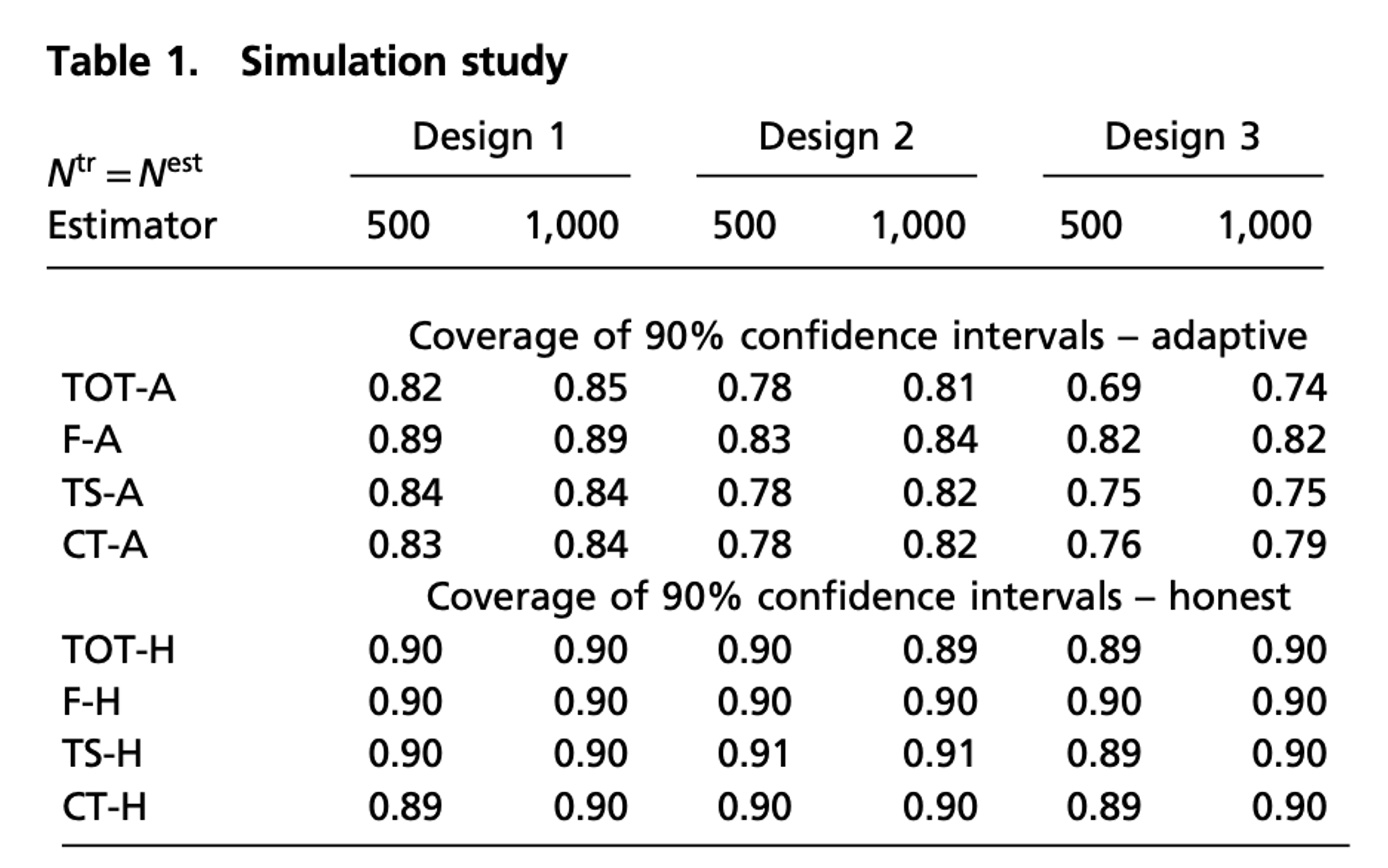
Goal: Compare the performance of proposed algorithms (Adaptive vs. Honest)

  • Evaluate Mean Squared Error (MSE) for each method
  • Evaluate 90% confidence interval coverage for each method
Notation Sample Size Role
N_tr 500 or 1,000 Tree Construction
N_est 500 (honest setting) Treatment Effect Estimation
N_te 8,000 Test Sample (MSE eval.)

Y_i(w) = \eta(X_i) + \frac{1}{2}\cdot (2w-1) \cdot {\color{red} \kappa (X_i)} + \epsilon_i

  • \epsilon_i \sim N(0,.01)
  • X_i \sim N(0,1)
  • \epsilon_i\perp X_i \quad \text{and}\quad X_i\perp X_j

We have three different setups:

  1. K=2; \quad \kappa(x) = \frac{1}{2}x_1
  2. K=10; \quad \kappa(x) = \sum_{k=1}^2 \mathbb{I}\{x_k >0\}\cdot x_k
  3. K=20; \quad \kappa(x) = \sum_{k=1}^4 \mathbb{I}\{x_k>0\} \cdot x_k
  • Design 1: two covariates. HTE is linear.
  • Design 2: six covariates. HTE is non linear
  • Design 3: eight covariates. HTE is non linear

Simulation Study: Results

CT-H vs alternative estimators

MSE divided by CT-H’s MSE
  • CT-H:
    • Best overall performance across all designs
  • F-H:
    • Performs worst in all designs; splits based on outcome prediction

Simulation Study: Results

Adaptive vs Honest : Coverage for 90% confidence intervals

Coverage of 90% confidence intervals
  • Honest estimation achieves nominal 90% coverage in all designs, while adaptive methods often fall below
  • The fit estimator has the highest adaptive coverage rates; it doesn’t focus on treatment effects
  • Honest estimation sacrifices some goodness of fit for valid confidence intervals

More results

Conclusion

  • By having a separate estimation set, tree-based ML approach can be used for estimating and testing heterogeneous treatment effects!
  • It imposes no restrictions on model complexity or the number of covariates, which helps setting data-driven hypotheses.
  • Different criterions can be used(fit, T-squared, etc.), but our baseline estimator(CT-H) performs the best in simulation.

Resources

Appendix

Cost and Benefits of Honest

  • Cost
    • Shallower tree (\because smaller leaves \rightarrow higher \mathbb{V})
    • Smaller # of samples \rightarrow Less personalized predictions and lower MSE
  • Benefit
    • EASY

    • Holding tree from \mathcal{S}^{\color{red}tr} fixed, can use standard methods to conduct inference (confidence interval) within each leaf of the tree on \mathcal{S}^{\color{red}te}

    (Disregard of the dimension of covariates)
    • No assumption on sparsity needed (c.f. nonparametric methods)
  • vs Dishonest with double the sample
    • Honest does worse if true model is sparse (also the case where bias is less severe)
    • Dishonest has similar or better MSE in many cases, but poor coverage of confidence intervals

Return

FAQ

  • Individuals on the edges of a leaf(outliers)
    • Use different method (e.g. Radom Forest) to provide a more personalized estimation. Causal Tree is to answer questions on the relation between covariates and how they interplay with treatment effects.
  • Is smaller number of samples bad?
    • Again, we’ve moved the goal post here. We are not trying to give the best prediction of effect on individuals. Rather, recursive partitioning assists figuring a general relation between covariates and treatment effects.
  • Why 50:50 in sample splitting?
    • Sample ratio could be taken differently in different problems and data available.

Simulation Study: Results

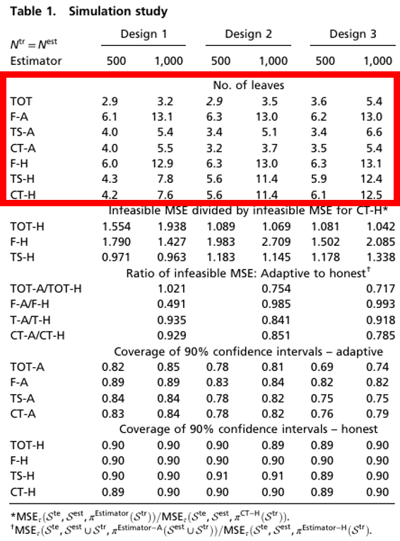
Number of Leaves(Tree Depth)

  • CT-H:
    • Splitting criteria: Maximizes – MSE
  • F-H:
    • Splitting criteria: Maximizes outcome prediction
    • Build deeper trees than that of CT
    • Less prone to overfitting on treatment effects
  • TS-H:
    • Splitting criteria: Maximizes squared t-statistic
    • Tree depth similar to that of CT
    • Adaptive versions still prone to overfitting

Simulation Study: Results

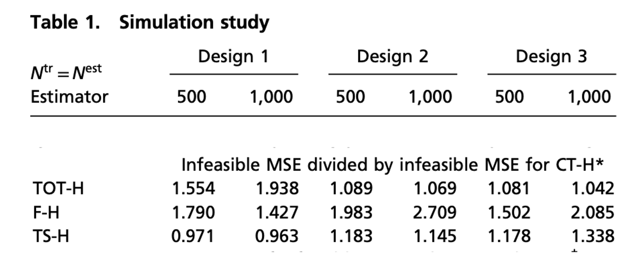
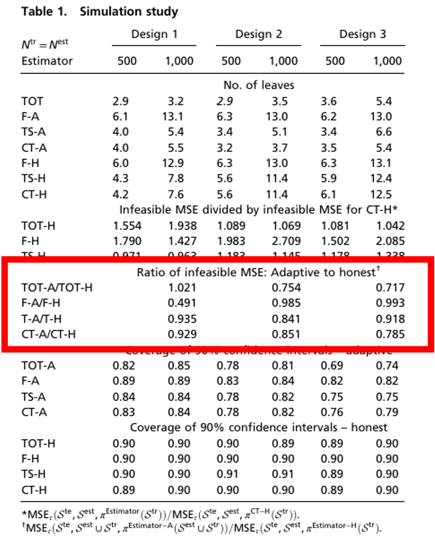
Adaptive vs Honest : Ratio of infeasible MSE

  • Honest estimation shows higher MSE in most cases \rightarrow Uses only half the data, leading to lower precision
  • Fit estimator performs poorly in Design 1 \rightarrow With smaller sample size, it tends to ignore treatment heterogeneity
  • As design complexity increases, the MSE ratio decreases. \rightarrow Adaptive estimators overfit more in complex settings.

Return